|
|
10.2
Pixels and Bits
Occasionally it will be useful to
remember that pixels—whether those seen on your computer screen or
those in the underlying image—are represented by bits. For those having only a
moderate understanding of computer architecture, a very brief
introduction to bits and color representation will be worthwhile.
A bit is
the fundamental unit of storage in a digital computer. There are
only two numeric values that can be stored in a single bit: 0 and
1. A ’0’ bit
represents the number zero, and a ’1’ bit represents the number
one. To represent numbers greater than one, we need to use
multiple bits in combination. For example, the number 1001001 in
binary represents the number 73 in decimal (decimal is the number system that
we use in everyday life, while binary
is the number system used internally by computers). For a given
number of bits, say eight, there is a smallest
number that can be
represented, and a largest
number that can be represented. The smallest 8-bit binary
number (in the encoding most often used for representing colors) is
00000000, which represents zero, while the largest is 11111111, which
represents 255. Thus, given only eight bits, we can represent
only 256 different numbers: 0, 1, 2, 3, 4, ... , 252, 253, 254, and
255. A 16-bit binary number, on the other hand, can
represent the whole numbers between 0 and 65535, which is a vastly
larger
range than 0 to 255, even though sixteen bits is only twice as many
bits as eight.
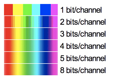 Fig.
10.2.1: Bits per channel. Each pixel is encoded via blending of
three channels: red,
Fig.
10.2.1: Bits per channel. Each pixel is encoded via blending of
three channels: red,
green, and blue. Each additional bit available for encoding pixel
colors doubles the
number of hues that can be specified. Using more bits can result
in smoother color gradients.
The practical consequence of this is that 16-bit
images enjoy a much, much larger color space than their 8-bit
counterparts, and therefore offer both greater color fidelity and
greater resiliance to the accumulation of certain artifacts that can
show up in the image after repeated use of certain postprocessing
operations. As we’ll see shortly, many image processing tasks
involve stretching the image’s histogram in various ways (histograms were introduced in
section 2.6), and this stretching can cause
visible artifacts in the
image; the occurrence of these artifacts is often greatly reduced by
simply working in a 16-bit color space rather than 8-bit. We’ll
show how to do that shortly. First, let’s consider some concrete
examples of how bit depth (number of bits per channel used to
encode an image) can affect image quality.
In the figure below we show a warbler image rendered
in 1, 2, 3, 4, 5, and 8 bits per
channel. The per channel
part refers to the fact that RGB images have three distinct channels: red, green, and blue (hence RGB). These three
channels get blended together to produce the other colors of the
rainbow that are needed in order to render a full-spectrum image.
As you’ll notice below, larger numbers of bits lend a very definite
improvement to image quality.
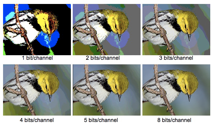 Fig.
10.2.2: Using more bits can result not only in smoother color
Fig.
10.2.2: Using more bits can result not only in smoother color
gradients in background regions, but also more details in the bird,
since details are encoded via finely-scaled color differentials.
For the first image, at 1 bit per channel, there are a total of three
bits (one each for the red, green, and blue channels). Because
each bit can only be in the 0 or 1 state, and because the three bits
can vary independently, there are a total of 23 = 8
different color hues that can be rendered; as is attested by the image
above, this isn’t enough hues to produce an aesthetically pleasing
image. In the second and third images (2 and 3 bits per channel),
there are significantly more details visible, and the colors begin to
approach what we’d expect to see in nature, though the backgrounds are
severely banded, due to what we call posterization.
As we’ll see shortly, posterization can be a problem even when a
relatively large number of bits are used to encode the image.
Note especially the difference in background
smoothness for the 5 bits-per-channel and 8 bits-per-channel images in
the figure above. For the 5 bits-per-channel imagte, it’s still
possible to see banding, or posterization, in the background regions of
the image, while for the 8 bit image the banding should be nonexistent
on most computer screens. The most important concept to
understand here is that for a given image, a larger number of bits can
give rise to appreciably smoother background gradients than some
smaller number of bits, and also more subtle details in the bird.
As we’ll see shortly, this issue comes into play not only for smaller
numbers of bits, but also for images that have been subjected to
certain forms of digital manipulations (especially repeated
applications of those digital manipulations), since some postprocessing
operations reduce the effective bit
utilization even when many bits are technically available in the
color space.
Before we continue, we need to review the definition
of a histogram. In the
following figure we show a photograph with its intensity histogram plotted in the
lower-left corner. The horizontal (x) axis of this graph corresponds
to pixel brightness, while the vertical (y) axis corresponds to the
frequency, or prevalence, of each brightness in the image. That
means that for a given pixel brightness measure (position along the x-axis), the height of the graph at
that point indicates how many pixels in the image have that
brightness.
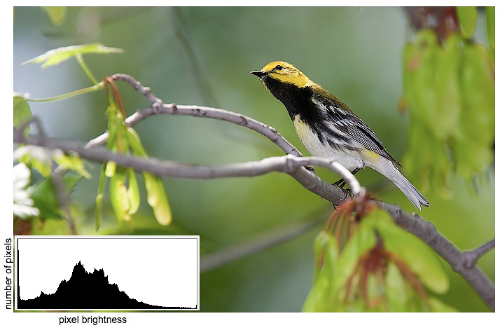
Fig. 10.2.3:
An image and its histogram. The horizontal
axis of the histogram corresponds to
pixel brightness; the vertical axis indicates the relative number of
pixels in the image that have that
brightness. Many postprocessing operations affect the
histogram. A large spike at either end of the
histogram indicates clipping, which can result in loss of detail.
In this particular example, the histogram indicates that most of the
image pixels are of medium brightness, though the left tail of the
distribution is fatter than the right tail, indicating a slight bias
toward the prevalence of darker pixels in the image. Notice also
that there is a peak in the graph right at the leftmost edge of the
histogram, indicating that some clipping of dark colors has occurred
(most likely in this warbler’s black throat patch, where details have
been largely obliterated due to the clipping). A much smaller
peak at the rightmost edge of the graph indicates a tiny amount of
clipping of detail in bright regions, which in this case appears to be
entirely negligible. Except for the issue of clipping, I almost
never consult the histogram during post-processing (or even when
shooting in the field—though I do rely crucially on my camera’s
blinking highlight alerts).
However, observing the effects of various post-processing operations on
the histogram can be very useful as you begin to learn about the many
caveats involved in applying these various operations.
In the figure below we show a histogram similar to
the one from the previous figure, but this time we also show the
per-channel (red, green, blue) decomposition below the main
histogram. As you can see, the clipping at the leftmost end of
the spectrum is confined to the blue channel. Depending on the
image you’re processing and the distribution of colors among the
subject and background regions of the image, you may or may not care
whether the blue channel (for example) is clipped at the left (or
right). The point is that when clipping is observed in the
composite histogram, you may want to view the individual channels to
see exactly what’s going on. As we’ll see in succeeding chapters,
repairing clipped shadows or highlights is sometimes possible, though
with greater or lesser amounts of effort, depending on the amount and
location (in the image) of the clipping.
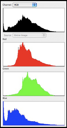
Fig. 10.2.4:
Color components of a histogram. Top: the composite
histogram.
Bottom three panes: red, green, and blue components making up the
composite
histogram. In this example the blue channel is clipped at the
left end.
In the histograms shown above, the x-axis was said to represent pixel intensity (meaning
brightness). You can also think of individual points along the x-axis as corresponding to
particular bit combinations—i.e., particular binary numbers encoding
pixel intensities in the three RGB channels. Keep this in mind as
you consider the histograms for the two images shown in the figure
below. The top part of the figure shows an image before a Levels operation is applied (in
Photoshop), while the bottom shows the image after the operation has
completed.
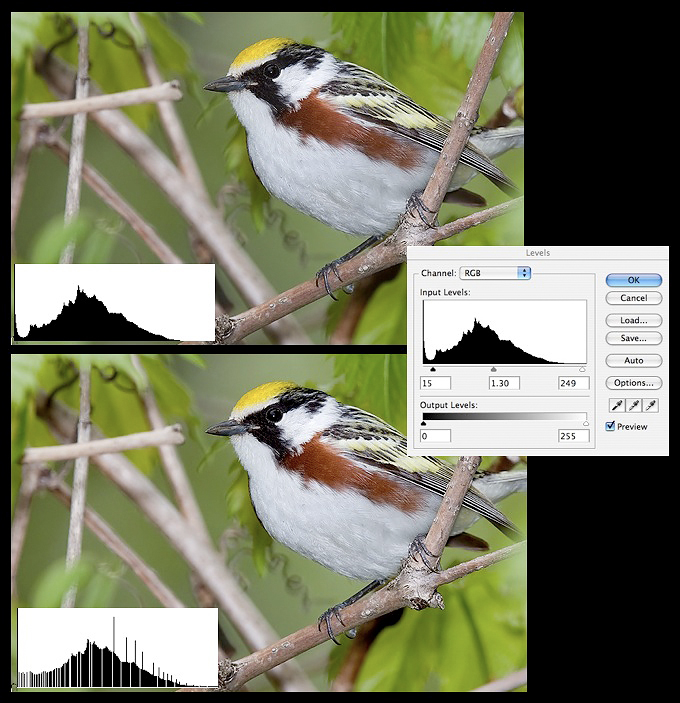
Fig. 10.2.5:
Histogram fragmentation. Top: an image before histogram
adjustment.
Right: stretching the histogram via the Levels tool in Photoshop.
Bottom: the image
after the adjustment. Notice the white gaps in the histogram;
these indicate ranges
of pixel values that are not used in the image. Successive
operations can widen these
gaps. If they get wide enough, the result can be visible
posterization—obvious color
discontinuities in regions of the image that should appear smooth (not
shown here).
As you can see, the bottom image
is somewhat brighter, and on some monitors may look a bit more
pleasing. However, the histogram for the bottom image has some
disturbing characteristics. Whereas the top image’s histogram is
relatively smooth and continuous, the bottom histogram is fragmented due to the insertion of
gaps in the graph. These gaps correspond to bit combinations that
do not occur anywhere in the image—that is, they represent colors (or
in this case intensities) that aren’t used in the image. For a
small number of such missing colors, the image aesthetics may be
entirely unaffected, especially for small print sizes. However,
as more image manipulations are performed and as these thin slices turn
into wide valleys of missing colors/intensities in the histogram,
visual manifestations can appear in the form of posterization.
While the image may still technically be encoded in 8 or 16 bits, those
bits are not being fully utilized, because some (perhaps many) bit
combinations are going unused. As noted earlier, posterization
typically shows up in background regions of an image that should
feature a smooth gradient, but instead appear choppy and banded.
What causes this effect? In short, image
processing causes it. Because there are only a fixed number of
discrete “bins” into which pixel values can fall,
and because image processing works by manipulating these hues and
therefore moving pixels from one bin to another, there is always the
potential to adversely affect the overall distribution of pixel hues
(i.e., the histogram). The main culprits, however, are exposure
transformations (such as Levels
and Curves in Photoshop) that
stretch or compress portions of the histogram. A useful mental
exercise is to consider what would happen if you first apply a
transformation that would compress the histogram into half its width,
and then expand it back to its original extent. Because of the
discrete nature of histogram bins, when the histogram is expanded back
to its original range you’d see a considerable loss of continuity in
the histogram.
At this point it’s worth revisiting a related issue
that was noted much earlier in this book: the fact that brighter pixels
are encoded with more bits (on average) than darker pixels. This
was one of the justifications for the ETTR (Expose To The Right) and BETTR (Bird Exposed To The Right)
philosophies expounded earlier (section 6.2).
In the histograms
shown above, each pixel intensity was represented by a point on the
horizontal (x) axis of the
histogram. In the computer, this axis is split into a small
number of bins, or
intervals. All of the pixel intensities falling in a single bin
share the same number of bits in their encoding, but different bins use
different numbers of bits for their pixels. What’s important here
is that bins further to the right on the histogram use more bits for
their pixels than bins further to the left, so they can represent more
distinct color shades. Each additional bit used in pixel
encodings doubles the number of color shades (hues) that can be
represented. Now, consider what happens when you underexpose an
image and then try to compensate for the underexposure by increasing
the brightness via software. Pixels from darker bins will be
re-mapped to lighter bins, as desired, but groups of pixels moved into
the brighter bins won’t magically experience a gain of information: if
there were only 32 different values represented in that dark bin, there
will still be only 32 different values when they get re-mapped to the
lighter bin, even if the lighter bin is capable of representing 64
distinct values. In this case we again have poor bit
utilization. This is why it’s better to expose to the right (in
the camera): if you later need to darken the image in software, pixels
will be moving from light bins to darker bins, and there won’t be any
information deficit involved in performing that mapping (just make sure
you don’t clip the highlights!). But going the other way
(brightening dark pixels artificially) often produces unpleasant image
artifacts, such as posterization or noise.
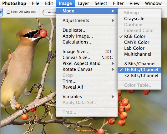
Fig. 10.2.6:
Working in 16 bit mode can be useful even if your original
image is only 8-bit (i.e., JPEG), because it reduces the magnitude and
impact of rounding errors in the computer.
One thing you can do to maximize the number of bits
available to you is to shoot in RAW instead of JPEG. Whereas JPEG
encodes images using only 8 bits per channel, most cameras’ RAW formats
utilize 12 or 14 bits per channel. When these are imported into
Photoshop, they’ll be represented internally in 16 bits per
channel. Note that even if your original image is an 8-bit JPEG,
it can be useful to convert it to a 16-bit file before performing your
postprocessing. As shown in the figure above, converting to
16-bit is as easy as selecting a menu option in Photoshop.
Converting an 8-bit image to 16-bit doesn’t actually add any more
information to the image, but it does give the computer more “headroom” for working with the image when
performing mathematical transformations on the pixel values. Many
people have found that this reduces the incidence of
posterization. Although there are a few operations that Photoshop
can only perform in 8-bit, I’ve rarely found that to be a problem; you
can always convert back to 8-bit via the same menu in Photoshop if
necessary.
An additional thing to note about JPEG files is that
they utilize a lossy compression
scheme, which can result in loss of image information during the
conversion to JPEG. If, for example, you convert a RAW image to
8-bit format, or if you load an image from an 8-bit TIFF file, and then
save it as a JPEG file, when you load the JPEG back into Photoshop
later you might notice some subtle distortions as compared to the
original uncompressed 8-bit image. JPEG files are typically ideal
for images that are to be displayed on a web page (i.e., on the
internet), because the compression scheme which they utilize often
results in small file sizes and therefore fast data transfer over the
internet. For your personal image archives, however, I recommend
using either RAW files or some other lossless format such as TIFF (or
Photoshop’s proprietary format, PSD). These files will be larger
and will therefore fill up your computer’s hard drive faster, but just
remember that larger files have more bits, and more bits means more
information (or at least the potential for more information).
Let's now very briefly revisit the issue
of color spaces. As
mentioned earlier, when working in an RGB color space, each pixel is
encoded by some number of bits (typically 8 or 16) per channel, with
the three channels being red, green, and blue. In other color
spaces (such as CMYK), colors will generally be encoded using a
different mapping, so that a particular bit string (e.g.,
1011101001011011) may encode a completely different color in different
color spaces. Photoshop renders this issue largely transparent,
since it converts the bit representations automatically for you when
you switch between color spaces, but it’s worthwhile to at least be
aware of the fact that a single bit encoding for a pixel can represent
either subtly or drastically different colors in different color
spaces. One context in which this becomes a practical issue is
when dealing with different computer platforms and rendering
devices. One image may appear lighter or darker, or more or less saturated (see section 10.4) on two
different computer systems, due to the slightly different ways in which
those systems map pixel values to actual colors. This is of
particular concern for users of Apple Macintosh computers, which, prior
to OS X version 10.6, applied a different gamma transformation to images
before displaying them than most other computer systems; the issue of
gamma is discussed in section 16.2.4.
Finally, it’s worthwhile at this juncture to refine
a concept introduced much earlier in this book. In section 2.5 we
described how photons are collected by the silicon photosites that
reside on the imaging sensor, and how these photons are counted and
their counts converted into analog pixel intensity signals that are
then converted into digital numbers and stored on the memory
card. What we didn’t explain was how colors are detected and
represented. Briefly, each photon, which can be interpreted
equivalently as an electromagnetic wave of a particular frequency,
encodes a particular value in the frequency spectrum. The
biological apparatus in the human eye and brain converts these
frequencies into what we perceive psychologically as colors. To
achieve this conversion (of frequency into color) in a digital sensor,
engineers have come up with a solution based on what’s known as the Bayer pattern, which is illustrated
below. This pattern would be repeated across the imaging sensor
so as to cover all photosites.
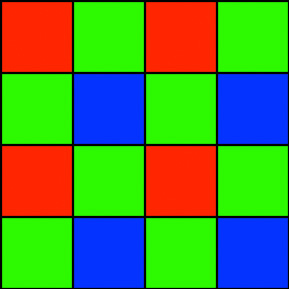
Fig. 10.2.7: The Bayer pattern.
Different photosites in a Bayer-style sensor
measure only one primary color. Interpolating
these into continuous pixel values is the job of the
demosaicing algorithm which is applied later
during RAW conversion. Note that the pattern
shown in this figure would be repeated across
the sensor so that each cell corresponds to one
photosite.
Each cell in the Bayer pattern corresponds to
one photosite. The color of a cell indicates which frequencies
are permitted to pass through the Bayer filter into the photosite lying
beneath the cell. Thus, red photosites count only those photons
having a frequency that falls within (what humans perceive as) the red
portion of the color spectrum, and similarly for the blue and green
sites. This of course reduces sample sizes and therefore
introduces a potential source of noise. More relevant to the
current discussion is the fact that only three colors are registered
under a Bayer system: pure red, pure green, and pure blue. In
order to reconstruct an image comprised of many different shades and
hues, an algorithm has to be applied which interpolates between the
neighboring red, green, and blue intensities measured under the Bayer
pattern. This process is referred to as demosaicing, and has a number of
subtle implications. For example, since noise may be more
prevalant in one of the three channels than the others, de-noising
algorithms operating on the RAW Bayer values can be more effective than
those applied to the post-interpolation data. The important point
is that RAW files contain the original red, green, and blue values
measured directly from the Bayer pattern (after ISO amplification and
digitization), and therefore contain more information than even a
high-bit TIFF file. As we’ll see in the next chapter, this is one
of the reasons why it’s beneficial to perform certain image processing
tasks during RAW conversion, rather than post-conversion.
Though the Bayer pattern is currently dominant among
consumer imaging devices, other patterns are in use and/or currently
under development. One such pattern splits the red, green, and
blue channels into three spatially separated layers of silicon.
Other patterns permit the binning
(pooling) of photon counts between neighboring photosites to reduce
sampling error and therefore reduce noise, at the cost of resolution.
|
|
|